Zaniar Shokati

Image classification is a type of supervised machine learning task where the goal is to sort images in a dataset into their appropriate categories or labels. For instance, classifying different types of dog breeds from images is a common example of image classification. This is referred to as “multi-class classification” since we’re sorting images into multiple categories. In this article, we’ll show you how to accomplish this using a pre-trained model called InceptionResNetV2, and how to customize it for your specific needs.

Transfer learning is a machine learning technique where a model developed for one task is reused as the starting point for a model on a second task. This is done by taking the weights of the pre-trained model and using them as the initial weights for the new model. The new model is then fine-tuned on the data for the second task.

Transfer learning is often used for image classification tasks, where pre-trained models such as InceptionResNetV2 and ResNet50 have been shown to achieve high accuracy on a variety of datasets.

Here is an example of how transfer learning can be used for dog breed classification:

1. Train a model on a large dataset of images from different dog breeds.
2. Fine-tune the model on a smaller dataset of images from the specific dog breeds that you are interested in classifying.
3. Use the fine-tuned model to predict the breed of new dog images.

The fine-tuned model is likely to perform better than a model that is trained from scratch on the smaller dataset of dog breed images. This is because the fine-tuned model has already learned the general features of images, such as edges and textures, from the pre-training dataset. All it needs to do is learn the specific features of the dog breed images to achieve high accuracy.

Transfer learning can be a very effective way to improve the performance of machine learning models, especially for tasks where there is limited training data available.

Here are some of the benefits of using transfer learning:

• It can save time and resources, as you do not need to train a model from scratch.
• It can improve the performance of machine learning models, especially for tasks where there is limited training data available.
• It can allow you to use machine learning to solve problems that would be difficult or impossible to solve without transfer learning.

InceptionResNetV2 is a convolutional neural network (CNN) architecture that was introduced in 2016 by Google. It is a variant of the Inception architecture that incorporates residual connections. Inception models use a set of filters of different sizes to extract features from images, while ResNet models use skip connections to improve the flow of information through the network. InceptionResNetV2 combines these two ideas to create a powerful model that can be used for image classification.

InceptionResNetV2 is a deep learning model with 164 layers. It is trained on the ImageNet dataset, which contains over 14 million images and 1000 object categories. InceptionResNetV2 has achieved state-of-the-art results on a variety of image classification benchmarks.

Import Libraries

To start, we begin by importing all the required libraries:

import numpy as np
import pandas as pd
import matplotlib.pyplot as plt
import cv2

import tensorflow as tf
from tensorflow.keras.preprocessing.image import ImageDataGenerator
from tensorflow.keras.applications import InceptionResNetV2
from tensorflow.keras.models import Sequential
from tensorflow.keras.layers import BatchNormalization, GlobalAveragePooling2D, Dense, Dropout
from tensorflow.keras.callbacks import EarlyStopping
from tensorflow.keras.regularizers import l2

physical_devices = tf.config.experimental.list_physical_devices('GPU')
if len(physical_devices) > 0:
    tf.config.experimental.set_memory_growth(physical_devices[0], True)

# Suppress warnings
import warnings
warnings.filterwarnings('ignore')

Load datasets

We proceed by loading datasets and image folders:

# Define data paths
train_path = "train"
test_path = "test"

# Load labels and sample data
labels = pd.read_csv("labels.csv")
sample = pd.read_csv('sample_submission.csv')

We add the ‘.jpg’ extension to each ID. This step allows us to retrieve images from the folder more efficiently, as the image names and IDs match, making it easier to locate the images.

# Update file extensions
labels['id'] = labels['id'].apply(lambda id: id + '.jpg')
sample['id'] = sample['id'].apply(lambda id: id + '.jpg')

Augmenting data

Data augmentation is the process of creating new data points from existing data. This can be done by applying various transformations to the data, such as cropping, flipping, rotating, and adding noise. Data augmentation can be used to increase the size and diversity of a dataset, which can help to improve the performance of a machine learning model.

Data preprocessing is the process of preparing the data for training and testing. This may involve tasks such as converting the data to a specific format, cleaning the data, and normalizing the data. Data preprocessing is important for ensuring that the data is in a format that the machine learning model can understand and that the data is representative of the real-world data that the model will be used on.

The provided code creates two ImageDataGenerator objects: one for the training data and one for the validation data. The ImageDataGenerator objects are configured to perform the following transformations:

• Rescaling: The images are rescaled to have a range of values between 0 and 1. This is a common preprocessing step for image data.
• Horizontal flipping: The images are flipped horizontally with a 50% probability. This is a simple data augmentation technique that can help to increase the diversity of the training data.
• Validation split: The images are split into a training set and a validation set. The validation set will be used to evaluate the performance of the model during training.

The create_data_generator() function creates a data generator from an ImageDataGenerator object and a Pandas DataFrame. The data generator will yield batches of data from the DataFrame, applying the transformations specified in the ImageDataGenerator object.

The train_generator and validation_generator variables are data generators for the training data and validation data, respectively. These data generators can be used to train and evaluate a machine learning model.

# Data augmentation and preprocessing
gen = ImageDataGenerator(
    rescale=1./255.,
    horizontal_flip=True,
    validation_split=0.2
)

def create_data_generator(data_frame, subset):
    return gen.flow_from_dataframe(
        data_frame,
        directory=train_path,
        x_col='id',
        y_col='breed',
        subset=subset,
        color_mode="rgb",
        target_size=(331, 331),
        class_mode="categorical",
        batch_size=32,
        shuffle=True,
        seed=20
    )

train_generator = create_data_generator(labels, "training")
validation_generator = create_data_generator(labels, "validation")

Building our Model

In this crucial step, we build our neural convolutional model. We start by loading the InceptionResNetV2 architecture with pre-trained ImageNet weights as the base. We configure it to have an input shape of (331, 331, 3) and set its layers to be non-trainable to prevent weight updates during training.

Next, we create our model using TensorFlow’s Sequential API. Here’s a breakdown of the components used:

• Base Model: We incorporate the pre-trained InceptionResNetV2 as the base of our model.
• BatchNormalization: This layer normalizes the activations along mini-batches rather than the entire dataset. It helps accelerate training, allowing the use of higher learning rates, and ensures the mean output is close to 0 and the standard deviation is close to 1.
• GlobalAveragePooling2D: This operation takes a tensor with a size of (input width) x (input height) x (input channels) and calculates the average value of all elements across the entire matrix for each channel. It reduces the dimensionality of the images by reducing the number of pixels, resulting in a 1-dimensional tensor of size (input channels) as output.
• Dense Layers: These layers are fully connected neural network layers that follow the convolutional layers.
• Dropout Layer: A dropout layer randomly drops some neurons from the input unit to prevent overfitting. The value 0.5 indicates that 50% of neurons are dropped during training.

The model is designed to perform image classification tasks, particularly for categorizing images into 120 different classes using a softmax activation function.

# Build the model
base_model = InceptionResNetV2(
    include_top=False,
    weights='imagenet',
    input_shape=(331, 331, 3)
)
# Fine-tune the top layers of the base model
fine_tune_at = 150 # 164 layers  
for layer in base_model.layers[:fine_tune_at]:
    layer.trainable = False
# base_model.trainable = False

model = Sequential([
    base_model,
    BatchNormalization(renorm=True),
    GlobalAveragePooling2D(),
    Dense(512, activation='relu', kernel_regularizer=l2(0.01)),
    Dense(256, activation='relu', kernel_regularizer=l2(0.01)),
    Dropout(0.5),
    Dense(128, activation='relu', kernel_regularizer=l2(0.01)),
    Dense(120, activation='softmax')
])

A kernel regularizer is a technique used to penalize the model for having large weights. This can help to prevent overfitting and improve the generalization performance of the model.

The l2 regularizer penalizes the model for the squared magnitude of its weights. The 0.01 hyperparameter controls the strength of the regularization. A higher value of 0.01 will result in stronger regularization.

In general, it is a good idea to use kernel regularization in deep learning models. However, the optimal regularization strength will depend on the specific problem and dataset.

Which layer you should use will depend on your specific needs. If you are concerned about overfitting, then you should use the second layer with the kernel regularizer. However, if you are not sure whether kernel regularization is necessary, then you can start with the first layer and add kernel regularization later if needed.

Here are some additional things to consider:

• Kernel regularization can make the training process slower.
• Kernel regularization can reduce the accuracy of the model on the training set, but it can improve the accuracy of the model on the test set.
• The optimal regularization strength will depend on the specific problem and dataset. You can use hyperparameter tuning to find the optimal regularization strength for your model.

Compile the model

Before training our model, we must configure it using the model.compile() function. This step involves defining the loss function, optimizer, and evaluation metrics for making predictions.

Out code uses an exponential decay learning rate schedule. This means that the learning rate will be gradually reduced over the course of training.

There are several advantages to using an exponential decay learning rate schedule:

• It can help to prevent the model from overfitting.
• It can help to improve the convergence of the training process.
• It can help to improve the generalization performance of the model.

The optimal values for the decay_steps and decay_rate hyperparameters will depend on the specific problem and dataset. However, a common rule of thumb is to set decay_steps to the total number of training steps and decay_rate to 0.9.

If you are not sure whether to use an exponential decay learning rate schedule, then you can start with the first code snippet and add it later if needed.

Here are some additional things to consider:

• Exponential decay learning rate schedules can make the training process slower.
• You may need to experiment with different values for the decay_steps and decay_rate hyperparameters to find the optimal values for your model.
• You can use a learning rate scheduler callback to monitor the training process and adjust the learning rate as needed.

# Learning rate scheduling
initial_learning_rate = 0.001
lr_schedule = tf.keras.optimizers.schedules.ExponentialDecay(
    initial_learning_rate, decay_steps=10000, decay_rate=0.9
)
optimizer = tf.keras.optimizers.legacy.Adam(learning_rate=lr_schedule)


model.compile(optimizer=optimizer, loss='categorical_crossentropy', metrics=['accuracy'])

Defining callbacks

Early stopping is a technique used to stop training a machine learning model early if the validation loss does not improve for a certain number of epochs. This can help to prevent overfitting and improve the generalization performance of the model.

The EarlyStopping callback function in Keras takes a number of parameters as input, including:

• patience: The number of epochs without improvement after which training will be stopped.
• min_delta: The minimum change in the validation loss that is considered an improvement.
• restore_best_weights: Whether to restore the best model weights found during training.

The following code creates an EarlyStopping callback function with a patience of 10 epochs, a minimum delta of 0.001, and the restore_best_weights flag set to True:

# Early stopping callback
early = EarlyStopping(patience=10, min_delta=0.001, restore_best_weights=True)

Train the Model

Training the model involves determining a set of weight and bias values that result in a low average loss across all the training data. This process is all about optimizing the model’s parameters to make accurate predictions and reduce errors.

# Define batch size and steps per epoch
batch_size = 32
STEP_SIZE_TRAIN = train_generator.n // batch_size
STEP_SIZE_VALIDATION = validation_generator.n // batch_size

# Fit the model
history = model.fit(
    train_generator,
    steps_per_epoch=STEP_SIZE_TRAIN,
    validation_data=validation_generator,
    validation_steps=STEP_SIZE_VALIDATION,
    epochs=25,
    callbacks=[early]
)

Save the Model

You can save the model for future use. This allows you to preserve the trained model so you can use it later for making predictions on new data without having to retrain it.

model.save("Model.h5")

Visualising the Model’s Performance

Visualizing the model’s performance typically involves creating graphical representations or plots to better understand how well the model is performing. This can include visualizing metrics like accuracy, loss, and other relevant statistics to assess the model’s effectiveness.

# Plot results
def plot_history(history):
    plt.figure(figsize=(10, 16))
    plt.rcParams['figure.figsize'] = [16, 9]
    plt.rcParams['font.size'] = 14
    plt.rcParams['axes.grid'] = True
    plt.rcParams['figure.facecolor'] = 'white'

    # Accuracy
    plt.subplot(2, 1, 1)
    plt.plot(history.history['accuracy'], label='Training Accuracy')
    plt.plot(history.history['val_accuracy'], label='Validation Accuracy')
    plt.legend(loc='lower right')
    plt.ylabel('Accuracy')
    plt.title(f'\nTraining and Validation Accuracy.\nTrain Accuracy: {str(history.history["accuracy"][-1])}\nValidation Accuracy: {str(history.history["val_accuracy"][-1])}')

    # Loss
    plt.subplot(2, 1, 2)
    plt.plot(history.history['loss'], label='Training Loss')
    plt.plot(history.history['val_loss'], label='Validation Loss')
    plt.legend(loc='upper right')
    plt.ylabel('Cross Entropy')
    plt.title(f'Training and Validation Loss.\nTrain Loss: {str(history.history["loss"][-1])}\nValidation Loss: {str(history.history["val_loss"][-1])}')
    plt.xlabel('epoch')
    plt.tight_layout(pad=3.0)

plot_history(history)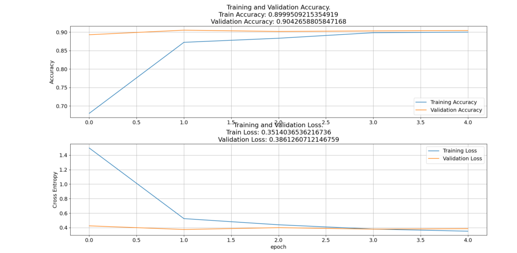

Evaluating the accuracy of the model

Evaluating the accuracy of the model means assessing how well the model performs on a given dataset. This typically involves measuring the model’s ability to make correct predictions, often expressed as a percentage or a metric like accuracy, precision, recall, or F1 score. The higher the accuracy, the better the model’s performance in making correct predictions.

# Evaluate the model
accuracy_score = model.evaluate(validation_generator)
print("Accuracy: {:.4f}%".format(accuracy_score[1] * 100))
print("Loss: ", accuracy_score[0])

Making predictions on the test data

Making predictions on the test data means using the trained model to generate output or predictions based on new, unseen data that was not used during the training process. This allows you to assess how well the model generalizes to new, real-world examples and evaluate its performance on data it has not encountered before.

# Make predictions and create a submission file
predictions = []
for image in sample.id:
    img = tf.keras.preprocessing.image.load_img(test_path + '/' + image)
    img = tf.keras.preprocessing.image.img_to_array(img)
    img = tf.keras.preprocessing.image.smart_resize(img, (331, 331))
    img = tf.reshape(img, (-1, 331, 331, 3))
    prediction = model.predict(img / 255)
    predictions.append(np.argmax(prediction))

my_submission = pd.DataFrame({'image_id': sample.id, 'label': predictions})
my_submission.to_csv('submission.csv', index=False)

You can download and inspect the implementation in this post in this GitHub repository .