Zaniar Shokati

We will explore the fascinating field of deep learning in this blog post. The primary neural network configuration we use today, feed-forward networks, will be the subject of our attention today. 

We will investigate the key ideas and theories that have shaped the deep learning field. In the upcoming posts, we’ll talk about the initial models and the concepts that underlie them while also introducing some theory and some implementation in Python. 

The Universal Function Approximation, which will show how neural networks can approximate any kind of function, is an important block that we will cover. The softmax function and a few activations will also be covered.

We sincerely hope that reading this blog post will help you learn more about the fascinating field of deep learning. Watch this space for more posts on this fascinating subject!

Perceptron

Perceptron is a fundamental building block of neural networks that are designed to mimic the functioning of the human brain. The perceptron is a single-layer neural network that is used to classify input data into two classes. It receives input from various sources, computes the weighted sum of inputs and passes it through an activation function to generate the output. Perceptron can model linear decision boundaries, meaning it can only solve linearly separable problems.

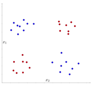
As a result, it is constrained in how well it can handle issues like the logical exclusive OR (XOR).  In the XOR problem, one class is represented by the top left and bottom right, while the other class is represented by the bottom left and top right. The logical XOR function served as inspiration for this. These two point clouds cannot be separated by a single linear decision boundary when they are visualized.

If the XOR problem cannot be solved, it implies that we lack the ability to describe the entire logic, which in turn means that achieving strong AI is not possible. This led to a period when funding for artificial intelligence research was drastically reduced, and researchers were unable to secure new grants to support their work. This period is commonly referred to as the “AI Winter.”

Multi-Layer Perceptron

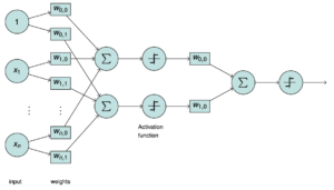
The introduction of the multi-layer perceptron marked a significant shift in the field of artificial neural networks. Rather than using a single neuron, the multi-layer perceptron employs multiple neurons arranged in layers. As shown in the simple diagram, the structure is similar to that of a perceptron, with inputs and weights. However, the difference lies in the multiple sums that go through non-linear functions, with the weights assigned and summarized again to go into another non-linearity.

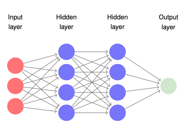
The ability to use multiple neurons in a multi-layer perceptron is highly intriguing since it enables the modeling of nonlinear decision boundaries. The neurons are arranged in hidden layers, meaning that they are not directly observing the input. Instead, they assign weights, perform computations, and only at the output layer, the results become visible. The weights that exist in the hidden layers are not directly observable, and their effects can only be seen when inputs are entered, and the activations are computed. At the output layer, we can observe the system’s behavior and understand what is happening. Therefore, the input layer, hidden layers, and output layer are critical components of the multi-layer perceptron.

Universal Function Approximator

A universal function approximator is a type of neural network that has the ability to approximate any kind of mathematical function. This is achieved through the use of multiple layers of neurons and weights, with non-linear activation functions applied at each layer. By adjusting the weights of the neural network, it is possible to fit the function to the given dataset with high accuracy. This concept is fundamental to the field of deep learning and has led to a paradigm shift in machine learning. Universal function approximators enable the modeling of complex relationships in data and have found applications in a wide range of domains, including computer vision, natural language processing, and robotics.

Softmax Activation Function

One-hot encoding is a technique used to represent categorical variables as numerical values. This technique involves converting each category into a binary vector, where each element in the vector corresponds to a possible category. The vector contains a 1 in the position that corresponds to the category and 0s in all other positions. This is useful for machine learning algorithms that require numerical inputs.

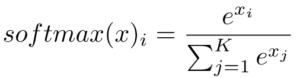
The softmax function is often used in conjunction with one hot encoding to generate a probability distribution over a set of possible outcomes. The softmax function takes as input a vector of numerical values, such as the output of a neural network, and converts them into a probability distribution. The function essentially normalizes the values in the input vector, ensuring that they sum up to 1. The resulting vector of probabilities can be used to make predictions or classify input data based on the most probable category. Together, one hot encoding and the softmax function are powerful tools for classification tasks in machine learning.

import numpy as np

class SoftMax:

    def __init__(self):
        self.y_hat = None

    def forward(self, input_tensor):
        max_row = np.max(input_tensor, axis=1, keepdims=True)
        input_tensor -= max_row

        ex_x = np.exp(input_tensor)
        sum_exp_x = np.sum(ex_x, axis=1, keepdims=True)
        self.y_hat = ex_x / sum_exp_x

        return self.y_hat

    def backward(self, error_tensor):
        error_tensor = self.y_hat * (error_tensor - np.sum(error_tensor * self.y_hat, axis=1, keepdims=True))
        return error_tensor

The SoftMax class has two methods, forward and backward. The forward method applies the Softmax activation function to its input tensor and returns the result. The backward method computes the derivative of the Softmax function and multiplies it with the error tensor to compute the error tensor for the previous layer.

Loss Function

In machine learning, the loss function is a key component of the training process for a model. The loss function measures the error between the predicted output of a model and the true output. The goal of the training process is to minimize the loss function, which means finding the model parameters that produce the smallest possible error between the predicted and true outputs. The choice of loss function is specific to the problem being solved and can vary widely depending on the type of data and the desired output. For example, a regression problem might use a mean squared error loss function, while a classification problem might use a cross-entropy loss function. The choice of loss function can have a significant impact on the performance of a model, and choosing an appropriate loss function is often a critical part of the modeling process.

import numpy as np

class CrossEntropyLoss:
    def __init__(self):
        self.y_hat = None

    def forward(self, input_tensor, label_tensor):
        self.y_hat = input_tensor
        mask = label_tensor == 1
        loss = np.sum(-1 * np.log(self.y_hat + np.finfo(float).eps) * mask)
        return loss

    def backward(self, label_tensor):
        error_tensor = np.divide(np.multiply(-1.0, label_tensor), self.y_hat)
        return error_tensor

The CrossEntropyLoss class can be used as a loss function in a machine learning model that performs classification tasks. During the training process, the forward() method is called to compute the loss between the predicted and true labels, and the backward() method is used to compute the gradients of the loss with respect to the model parameters, which are then used to update the parameters through gradient descent or another optimization algorithm.

Training

One crucial aspect we haven’t addressed yet is the process of training neural networks. As previously discussed, the hidden layers of a neural network cannot be directly observed, which poses a significant challenge. Modifying any part of the processing chain can potentially disrupt the entire system, making it a complex task to adjust anything along the way. Therefore, it is essential to exercise caution and carefully consider all the other processing steps when making any modifications. The process of training neural networks requires careful adjustment of parameters and fine-tuning of the network architecture to ensure optimal performance while avoiding any adverse effects that may arise from even minor adjustments. To achieve an optimal set of weights, we select the approach of minimizing the loss function concerning weight over the complete training data set.

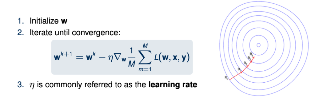
Gradient Descent

Gradient descent is an iterative optimization algorithm used to minimize the loss function of a machine learning model. It works by computing the gradient of the loss function with respect to the model’s parameters (usually the weights), and then adjusting the parameters in the opposite direction of the gradient to minimize the loss. The algorithm starts with an initial set of weights and iteratively updates them using the gradient of the loss function until the minimum of the function is reached. The size of the update in each iteration is controlled by a hyperparameter called the learning rate. If the learning rate is too small, the algorithm may converge slowly, while if it is too large, the algorithm may not converge at all or even diverge. There are several variations of gradient descent, such as stochastic gradient descent and batch gradient descent, which differ in how the gradient is computed and updated. Gradient descent is a fundamental optimization algorithm in machine learning and is widely used in various models such as neural networks and linear regression.

class Sgd:
    def __init__(self, learning_rate=0.01):
        self.learning_rate = learning_rate

    def calculate_update(self, weight_tensor, gradient_tensor):
        return weight_tensor - self.learning_rate * gradient_tensor

This code defines a Python class Sgd which implements the stochastic gradient descent (SGD) optimization algorithm commonly used in machine learning for updating the parameters of a model during training.

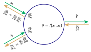
Backpropagation Algorithm

Backpropagation involves calculating the gradients of the loss function with respect to the weights of the network, which are then used to update the weights via gradient descent. The algorithm works by first forward propagating an input through the network to obtain a prediction. The difference between the prediction and the target output is then used to compute the loss function. The next step is to backpropagate the error through the network, starting from the output layer and moving backwards through the layers, to compute the gradient of the loss with respect to the weights. This is done using the chain rule of calculus, which allows the error to be propagated backwards through the network by computing the derivative of the activation function at each layer. The gradients are then used to update the weights via gradient descent. This process is repeated iteratively until the loss is minimized and the network is trained.

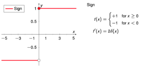
Sign Activation Function

The sign function is a mathematical function that takes an input and returns its sign as output, which is either +1 or -1, depending on whether the input is positive or negative. In the context of activation functions in neural networks, the sign function can be used as a binary activation function, where the output of a neuron is either +1 or -1 depending on whether the weighted sum of its inputs is greater than or less than zero, respectively.

However, the sign function is rarely used as an activation function in modern neural networks because of its discontinuous nature, which makes it difficult to optimize using gradient-based methods such as backpropagation. Additionally, its output is limited to binary values, which limits the expressive power of the neural network. Instead, continuous and differentiable activation functions such as the sigmoid, ReLU, and softmax functions are typically used in modern neural networks.

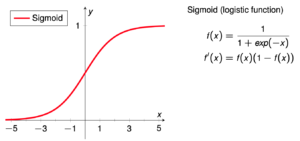
Smooth Activation Function (Sigmoid)

The sigmoid function is a smooth, S-shaped curve that takes an input and produces an output between 0 and 1. The sigmoid function has several desirable properties that make it a popular choice for neural network activation functions. Firstly, its output is always between 0 and 1, making it ideal for applications such as binary classification, where the output should represent a probability of a binary event occurring. Additionally, the sigmoid function is differentiable, which means it can be used with gradient-based optimization algorithms, such as backpropagation, to update the weights of a neural network during training. However, the sigmoid function has a vanishing gradient problem, which means that as the input becomes very large or very small, the gradient of the function approaches zero, making it difficult to train deep neural networks.

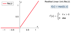
Rectified Linear Unit (ReLU)

The Rectified Linear Unit (ReLU) is a popular activation function used in neural networks. It has the form f(x) = max(0,x), where x is the input to the function. This means that any negative input will be set to 0, while positive inputs will be passed through unchanged. The ReLU function has several advantages over other activation functions. Firstly, it is computationally efficient to compute, since it involves only simple arithmetic operations. Secondly, it avoids the vanishing gradient problem that can occur with other activation functions, since it has a non-zero derivative for positive inputs. Finally, it has been shown to be effective in training deep neural networks, leading to improved performance on a variety of tasks.

import numpy as np

class ReLU:
    def __init__(self):
        self.input_tensor = None

    def forward(self, input_tensor):

        self.input_tensor = input_tensor
        self.input_tensor = np.maximum(0, self.input_tensor)
        return self.input_tensor

    def backward(self, error_tensor):
        input_mask = self.input_tensor > 0
        temp = error_tensor * input_mask
        return temp

The ReLU class has two methods, forward and backward. The forward method applies the ReLU activation function to its input tensor and returns the result. The backward method computes the derivative of the ReLU function and multiplies it with the error tensor to compute the error tensor for the previous layer.

Fully Connected Layer

A fully connected layer is a type of layer in a neural network where each neuron is connected to all neurons in the previous layer. This means that every output from the previous layer is an input to every neuron in the current layer. The fully connected layer is also known as a dense layer because of its high density of connections. The weights between the neurons in the fully connected layer are learned during the training process through backpropagation. Fully connected layers are commonly used in deep neural networks for tasks such as image classification and natural language processing. However, they can also lead to overfitting, where the model becomes too complex and is unable to generalize well to new data. To prevent overfitting, techniques such as regularization and dropout can be used.

import numpy as np

class FullyConnected:
    def __init__(self, input_size, output_size):
        self.weights = np.random.uniform(0, 1, size=(input_size + 1, output_size))  # changed Weights includes biases as well changed
        self.input_size = input_size
        self.output_size = output_size
        self._optimizer = None
        self.input_tensor = None
        self._gradient_weights = None

    def get_optimizer(self):
        return self._optimizer

    def set_optimizer(self, optimizer_value):
        self._optimizer = optimizer_value

    optimizer = property(get_optimizer, set_optimizer)

    def get_gradient_weights(self):
        return self._gradient_weights

    def set_gradient_weights(self, gradient_weights):
        self._gradient_weights = gradient_weights

    gradient_weights = property(get_gradient_weights, set_gradient_weights)

    def forward(self, input_tensor):
        temp = np.ones((np.shape(input_tensor)[0], 1))
        self.input_tensor = np.append(temp, input_tensor, axis=1)
        output = np.dot(self.input_tensor, self.weights)
        return output

    def backward(self, error_tensor):
        self.gradient_weights = np.dot(self.input_tensor.T, error_tensor)
        if self.optimizer is not None:
            self.weights = self._optimizer.calculate_update(self.weights, self.gradient_weights)

        error_tensor = np.dot(error_tensor, self.weights[1:, :].T)  # gradient_wrt_input

        return error_tensor

Conclusion

In conclusion, the fully connected neural network is a fundamental and widely used architecture in deep learning that has proven effective in solving a variety of complex problems. By leveraging the power of parallel computing and backpropagation, fully connected neural networks can learn complex relationships in data and make accurate predictions. While this architecture has limitations, such as scalability and overfitting, recent advancements in neural network research have addressed some of these challenges, making fully connected neural networks more powerful and versatile than ever before. As the field of deep learning continues to evolve, it is certain that fully connected neural networks will remain a vital tool in the machine learning toolkit.

You can download and inspect the implementation of mentioned layers in this post in this GitHub repository . Once you’ve reviewed the contents, feel free to share the link with others who may be interested. Happy exploring!